산업에서 Feedback Control System을 디자인할 때 Frequency-Response를 많이 활용한다고 한다. 특히 Plant model의 불확실성 면에서 좋은 디자인을 제공해줄 수 있다.
사인파 입력(sinusoidal inputs)에 대한 선형 시스템의 response를 그 시스템의 Frequency Response라 한다. 이는 pole and zero locations으로부터 알 수 있다.
we consider a system described by $$\frac{Y(s)}{U(s)}=G(s)$$ where the input $u(t)$ is a sine wave with an amplitude $A$: $$u(t)=A\sin(\omega_0t)1(t)$$
If all the poles of the system represent stable behavior (the real parts of $p_1, p_2, . . . , p_n < 0$), the natural unforced response will die out eventually, and therefore the steady-state response of the system will be due solely to the sinusoidal term.
Using cover-up method, $$\alpha_0=(s+j\omega_0)Y(s)|_{s=-j\omega_0}=G(-j\omega_0)\frac{A\omega_0}{-2j\omega_0}=-\frac{A}{2j}G(-j\omega_0)$$
num = [1 1];
den = [0.1 1];
sysD = tf(num, den);
w = logspace(-1, 2);

[mag, phase] = bode(sysD, w);

loglog(w, squeeze(mag)), grid;
semilogx(w, squeeze(phase)), grid;
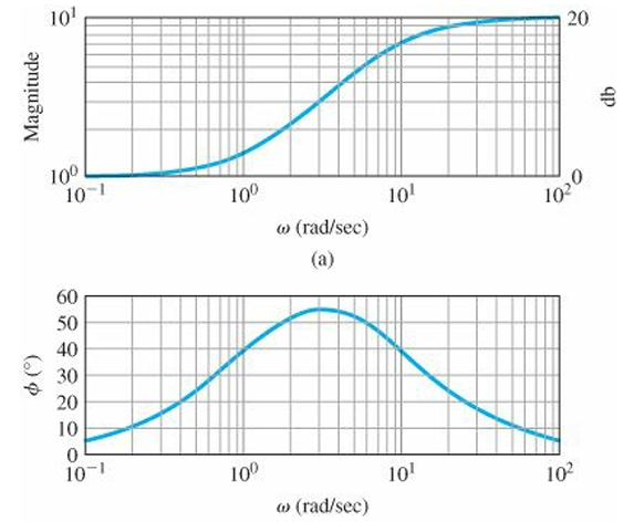
Magnitude는 low frequency일 때 $1(=K)$, high frequency일 때 $10(=K/\alpha)$인 것을 확인할 수 있다. Phase는 low and high frequency일 때 phase가 0에 가까워지고 중간 즈음의 frequency에서 높은 phase가 나타나는 것을 관찰할 수 있다.
Transfer Function에 대하여 frequency에 따른 Magnitude와 Phase는 시스템의 dynamic response에 대한 정보를 제공한다. sinusoid input에 대하여 $M$과 $\phi$는 response를 온전히 묘사할 수 있고, periodic input의 경우 푸리에 급수를 통해 sum of sinusoids로 분해하여 total response를 분석할 수 있다. transient input에 대하여는 $G(j\omega)$와 라플라스 변환을 통해 얻은 transient response 간의 관계를 통해 이해하는 것이 좋다.
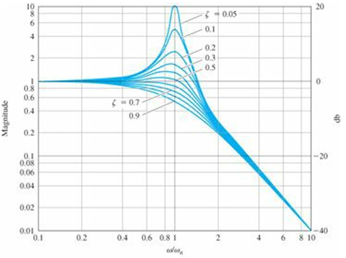
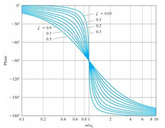
다음 전달함수를 생각해 보자. $$G(s)=\frac{1}{(s/\omega_n)^2+2\zeta(s/\omega_n)+1}$$
$\zeta$ 값에 따른 $M(\omega)$와 $\phi(\omega)$의 분포는 다음과 같다. 시스템의 damping이 transient response overshoot나 magnitude peak에 영향을 미치는 것을 관찰할 수 있다. 또한 $\omega_n$이 거의 bandwidth와 비슷하므로 bandwidth로부터 rise time을 추정할 수 있다. $\zeta<0.5$에서 peak overshoot이 약 $1/2\zeta$인 것도 확인할 수 있다.
Figure 6.3(a)Figure 6.3(b)
Bandwidth
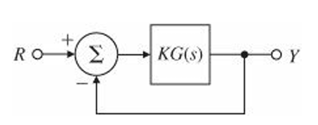
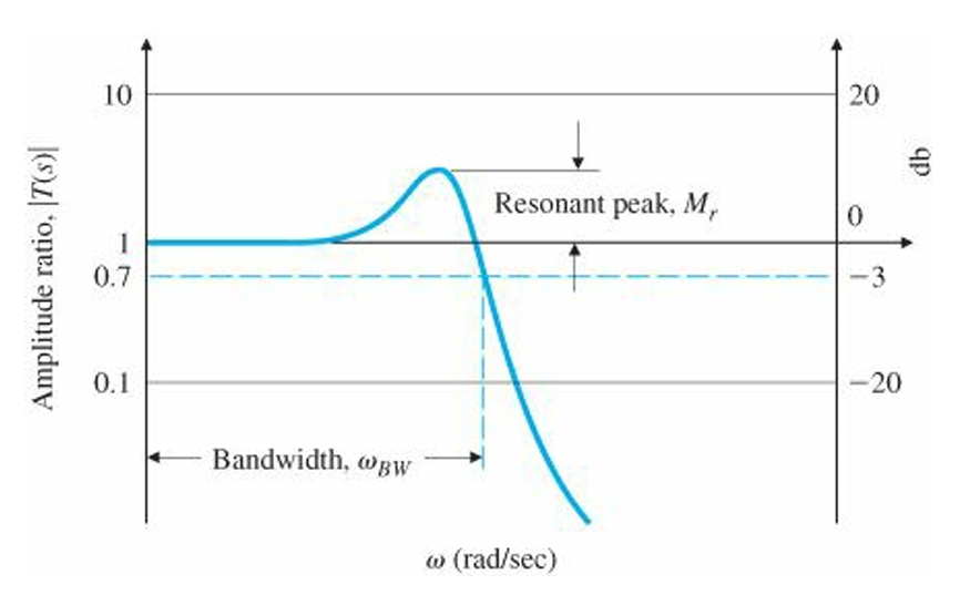
A natural specification for system performance in terms of frequency response is the bandwidth, defined to be the maximum frequency at which the output of a system will track an input sinusoid in a satisfactory manner. By convention, for the system with a sinusoidal input $r$, the bandwidth is the frequency of $r$ at which the output $y$ is attenuated to a factor of 0.707 times the input. $$\frac{Y(s)}{R(s)}\overset{\underset{\mathrm{def}}{}}{=}T(s)=\frac{KG(s)}{1+KG(s)}$$
Bandwidth is a measure of speed of response and is therefore similar to time-domain measures such as rise time and peak time or the s-plane measure of dominant-root(s) natural frequency. In fact, if the $KG(s)$ is such that the closed-loop response is given by the graphs above, we can see that the bandwidth will equal the natural frequency of the closed-loop root (that is, $\omega_{BW} = \omega_n$ for a closed-loop damping ratio of $\zeta = 0.7$). For other damping ratios, the bandwidth is approximately equal to the natural frequency of the closed-loop roots, with an error typically less than a factor of 2.
Bandwidth의 정의는 physical control system 등 low-pass filter behavior가 있는 시스템에 대하여 논할 때 의미가 있다. 그 외의 적용에 있어 Bandwidth는 다소 다르게 정의될 수 있다. 또한 high-frequency roll-off, 즉 고주파에서 값이 떨어지는 현상이 일어나지 않는 이상적인 시스템이라면 bandwidth는 무한대가 된다(e.g. # of poles = # of zeros).
Bode Plot
Magnitude curve는 log scale로, Phase curve는 linear scale로 그려 high-order system을 그릴 수 있다.
$$G(j\omega)=Me^{j\phi}=\frac{r_1e^{j\theta_1}r_2e^{j\theta_2}}{r_3e^{j\theta_3}r_4e^{j\theta_4}r_5e^{j\theta_5}}$$라 하자. 그러면 $$\left |G(j\omega) \right |=\frac{r_1r_2}{r_3r_4r_5},$$
where $$\log_{10}M=\log_{10}r_1+\log_{10}r_2-\log_{10}r_3-\log_{10}r_4-\log_{10}r_5$$
Power $P$, Voltage $V$에 대해서, $$\left |G \right |_{db}=10\log_{10}\frac{P_2}{P_1}=20\log_{10}\frac{V_2}{V_1}$$
따라서 Bode plot을 $\left |G \right |_{db}$ vs. $\log \omega$와 Phase (deg) vs. $\log \omega$ 로 표현할 수 있다. 이때 Magnitude에서 log를 씌워서 수직 방향 스케일이 db과 선형적이도록 표현하곤 한다.
Advantages of Bode plots
1. Dynamic compensator design can be based entirely on Bode plots.
2. Bode plots can be determined experimentally.
3. Bode plots of systems in series (or tandem) simply add, which is quite convenient.
4. The use of a log scale permits a much wider range of frequencies to be displayed on a single plot than is possible with linear scales.
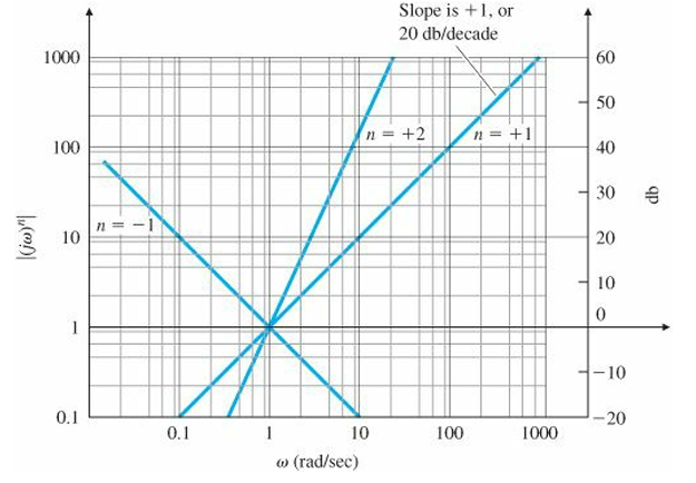
Magnitude Plot 기울기가 n x (20 db per decade)인 직선으로 그려지게 된다.
Class 2. $(j\omega\tau+1)^{\pm1}$
*first-order term
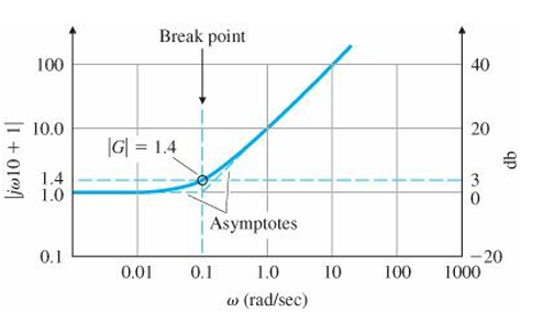
Magnitude Plot은 낮은 주파수일 때와 높은 주파수일 때 각각 다른 점근선(Asymptotes)을 갖는다.
For $\omega\tau\ll 1$, $j\omega\tau+1\cong 1$
For $\omega\tau\gg 1$, $j\omega\tau+1\cong j\omega\tau$
$\omega=1/\tau$를 break point라 칭한다. break point보다 작은 주파수에서는 magnitude가 거의 상수고 break point보다 큰 주파수에서는 Class 1과 유사한 양상을 보인다.
아래의 그림은 $\tau=10$일 때, 즉 $G(s)=10s+1$일 때의 magnitude plot이다. break point에서 점근선과 실제 곡선의 차이가 1.4 정도 (3 db) 있는 것을 관찰할 수 있다. break point 이전의 주파수에서는 거의 0 db이고, break point 이후의 주파수에서는 기울기가 +1(or +20 db per decade)이다.
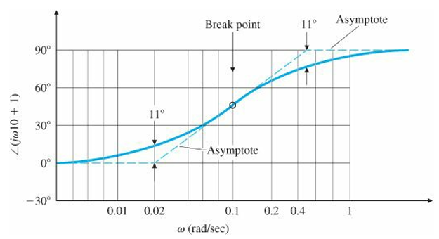
Phase는 주파수의 범위에 따라 점근선을 크게 세 개로 나눌 수 있다.
For $\omega\tau\ll 1$, $\angle 1=0^\circ$
For $\omega\tau\gg 1$, $\angle j\omega\tau=90^\circ$
For $\omega\tau\cong1$, $\angle (j\omega\tau+1)=45^\circ$
Class 3. $\left [ \frac{j\omega}{\omega_n}+2\zeta\frac{j\omega}{\omega_n}+1 \right ]^{\pm1}$
*second-order term
break point는 $\omega=\omega_n$으로 한다.
큰 양상은 Class 2와 유사하다. Magnitude는 break point로부터 기울기 +2(or +40 db per decade)를 갖는 직선 형태다. second-order term이 분모에 있다면 기울기는 -2다. Phase도 마찬가지로 Class 2의 두 배인 $\pm 180^{\circ}$로 변화한다.
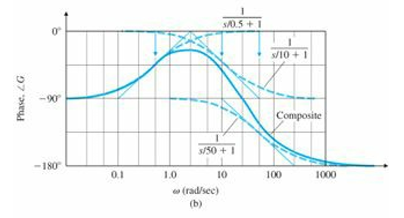
다만 damping ratio $\zeta$에 따라 break point 주변의 transition이 다르다. 위의 Figure 6.3에서 그 모습을 확인할 수 있다.
Peak Amplitude: Figure 6.3과 같이 second-order term이 분모에 있는 경우 Magnitude의 최댓값은 break point에서 발생하며 그 값은 $\left | G(j\omega_n)\right |=1/2\zeta$ 이다.
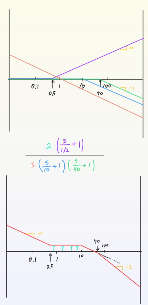
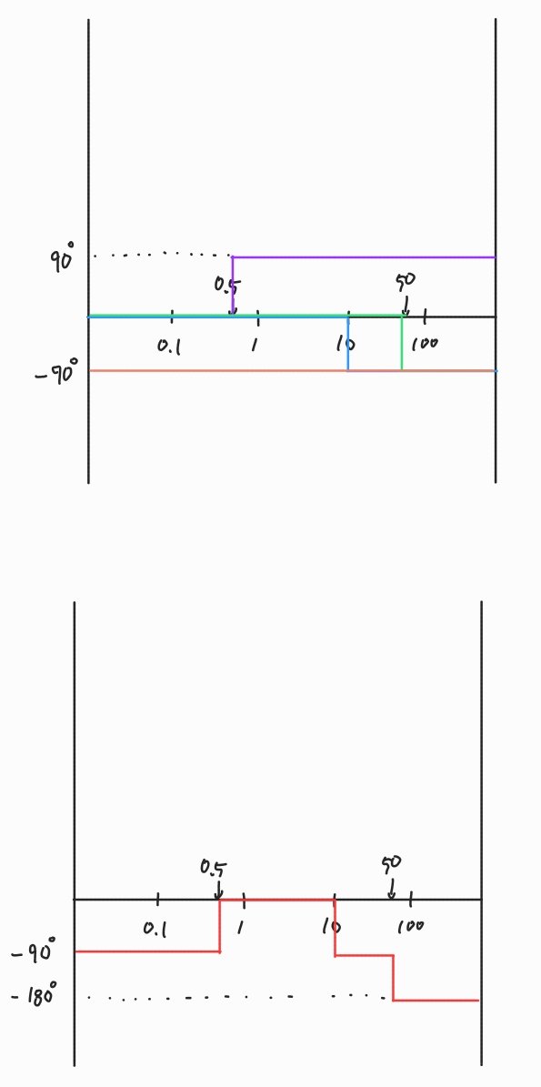
poles과 zeros가 여러 개 있는 시스템의 경우 frequency response는 각 component가 결합된 composite curve로 표현된다. Composite Magnitude Curve는 각 curve 점근선의 기울기를 합한 것이고, Composite Phase Curve는 각 curve를 그대로 합한 것이다. 이 규칙은 우선 LHP의 poles과 zeros에 대한 것이며 changes for singularities in RHP는 추후 고려하도록 한다.
ex 6.3)
다음 전달 함수의 Bode Plot을 그려보자. $$KG(s)=\frac{2000(s+0.5)}{s(s+10)(s+50)}$$
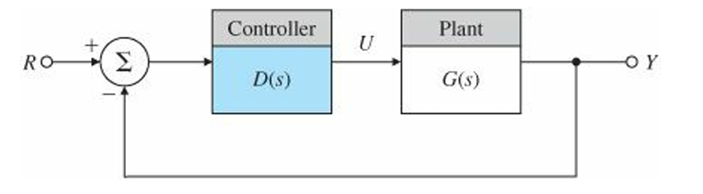
For this system, the closed-loop transfer function is $$\frac{Y(s)}{R(s)}=\frac{D(s)G(s)}{1+D(s)G(s)H(s)}$$ and the characteristic eqn, whose roots are the poles of this transfer function, is $$1+D(s)G(s)H(s)=0$$
Let the open loop transfer function $$L(s)=\frac{b(s)}{a(s)}$$
then the characteristic eqn: $$1+KL(s)=0$$
Evans's Method
If the parameter is the gain of the controller, then $L(s)$ is proportional to $D(s)G(s)H(s)$
Evans suggested that we plot the locus of all possible roots of $1+KL(s)=0$ as $K$ varies from zero to infinity and then use the resulting plot to aid us in selecting the best value of $K$. Also we can determine the consequences of additional dynamics added to $D(s)$ as compensation in the loop considering the effects of additional poles and zeros on this graph.
$$L(s)=\frac{b(s)}{a(s)}\quad where \quad b(s)=\prod_{i=1}^{m}(s-z_i),\quad a(s)=\prod_{i=1}^{n}(s-p_i)$$
Definition 1. The root locus is the set of values of s for which $1+KL(s)=0$ is satisfied as the real parameter $K$ varies from $0$ to $+\infty$. Typically, $1+KL(s)=0$ is the characteristic equation of the system, and in this case the roots on the locus are the closed-loop poles of that system.
Definition 2. The root locus of $L(s)$ is the set of points in the s-plane where the phase of $L(s)$ is 180˚. If we define the angle to the test point from a zero as $\psi_i$ and the angle to the test point from a pole as $\phi_i$ then Definition 2 is expressed as those points in the s-plane where, for integer $l$, $$\sum \psi_i-\sum\phi_i=180^{\circ}+360^{\circ}(l-1)$$
The immense merit of Definition 2 is that, while it is very difficult to solve a high-order polynomial by hand, computing the phase of a transfer function is relatively easy.
e.g.
$$L(s)=\frac{s+1}{s(s+5)[(s+2)^2+4]}$$
Mark poles and zeros on the s-plane. Suppose our test point is $s_0=-1+2j$. We would like to test whether or not $s_0$ lies on the root locus for some value of $K$.
Measuring the phase
we must have $\angle L(s_0)=180^{\circ}+360^{\circ}(l-1)$ for some integer $l$.
Since the phase of $L(s)$ is not $180 ^{\circ}$, we conclude that $s_0$ is not on the root locus.
Rules for Plotting a Positive($180 ^{\circ} $) Root Locus
Rule 1. The $n$ branches of the locus start at the poles of $L(s)$ and $m$ of these branches end on the zeros of $L(s)$.
Rule 2. The loci are on the real axis to the left of an add number of poles and zeros.
Rule 3. For large $s$ and $K$, $n-m$ of the loci are asymptotic to lines at angles $\phi_l$ radiating out from the point $s=\alpha$ on the real axis where $$\phi_l=\frac{180^{\circ}+360^{\circ}(l-1)}{n-m},\quad l=1,2,...,n-m,\quad\alpha=\frac{\sum p_i-\sum z_i}{n-m}$$
Rule 4. The angle(s) of departure of a branch of the locus from a pole of multiplicity q is given by $$q\phi_{l,dep}=\sum\psi_i-\sum_{i\neq l}^{}\phi_i-180^{\circ}-360^{\circ}(l-1)$$ and the angle(s) of arrival of a branch at a zero of multiplicity q is given by $$q\psi_{l,arr}=\sum\phi_i-\sum_{i\neq l}^{}\psi_i+180^{\circ}+360^{\circ}(l-1)$$
Rule 5. The locus can have multiple roots at points on the locus and the branches will approach a point of q roots at angles separated by $$\frac{180^{\circ}+360^{\circ}(l-1)}{q}$$ and will depart at angles with the same separation.
Selecting the Parameter Value
for $s_0$ on the Root Locus, $$K=-\frac{1}{L(s_0)}=\frac{1}{\left| L(s_0) \right|}$$
e.g.
PD Control with the plant of $$K=\frac{1}{L(s_0)}=\frac{1}{\left| L(s_0) \right|}$$
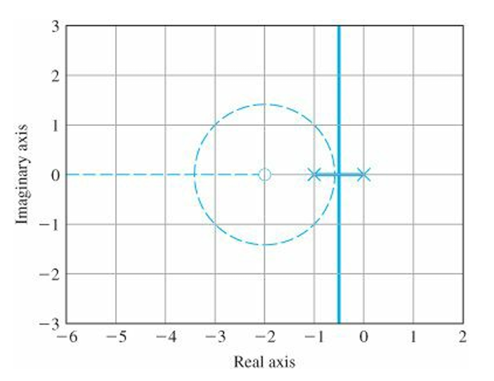
When the third pole is near the zero (p near 1), there is only a modest distortion of the locus that would result for $D(s)G(s)\cong K\frac{1}{s^2}$ which consists of two straight-line locus branches departing at $\pm90^\circ$ from the two poles at $s = 0$.
As we increase p, the locus changes until at $p = 9$ the locus breaks in at –3 in a triple multiple root.
As the pole p is moved to the left beyond –9, the locus exhibits distinct break-in and breakaway points, approaching, as p gets very large, the circular locus of one zero and two poles.
When p = 9, is thus a transition locus between the two second-order extremes, which occur at p = 1 (when the zero is canceled) and p → ∞ (where the extra pole has no effect).
Design using Dynamic Compensation
Lead compensation approximates the function of PD control and acts mainly to speed up a response by lowering rise time and decreasing the transient overshoot.
Lag compensation approximates the function of PI control and is usually used to improve the steady-state accuracy of the system.
Notch compensation will be used to achieve stability for systems with lightly damped flexible modes, as we saw with the satellite attitude control having noncollocated actuator and sensor.
Lead and Lag Compensation
$$D(s)=K\frac{s+z}{s+p}$$
Compensation with this transfer function is called Lead Compensation if $z<p$ and Lag Compensation if $z>p$.
Compensation is typically placed in series with the plant in the feed-forward path.
It can also be placed in the feedback path and in that location has the same effect on the overall system poles but results in different transient responses from reference inputs.
characteristic eqn: $$1+D(s)G(s)=1+KL(s)=0$$
Lead Compensation
e.g.
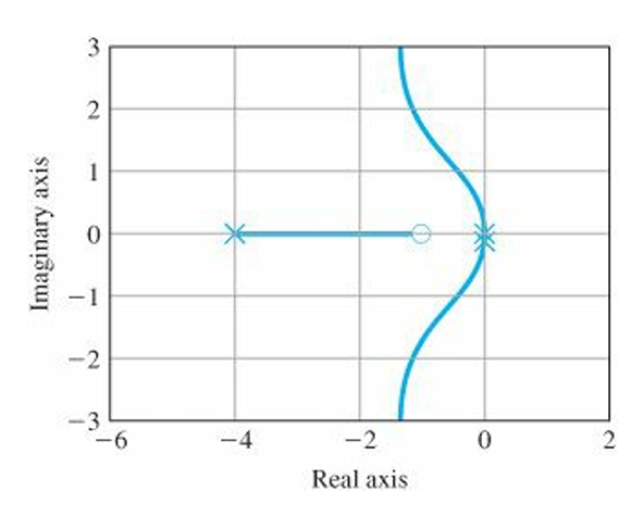
$$G(s)=\frac{1}{s(s+1)}$$
$D(s)=K$(solid) vs. $D(s)=K(s+2)$(dashed)
The effect of the zero is to move the locus to the left, toward the more stable part of the s-plane.
If our speed-of-response specification calls for $\omega_n=2$, then proportional control alone (D = K) can produce only a very low value of damping ratio $\zeta$ when the roots are put at the required value of $\omega_n$.
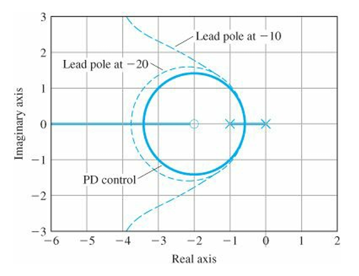
But, the pure derivative control is not normally practical because of the amplification of sensor noise implied by the differentiation and must be approximated. If the pole of the lead compensation is placed well outside the range of the design $\omega_n$, then we would not expect it to upset the dynamic response of the design in a serious way. $$D(s)=K\frac{s+2}{s+p}$$
Consider $p=10$ and $p=20$.
For small gains, before the real root departing from –p approaches –2, the loci with lead compensation are almost identical to the locus for pure PD. The effect of the pole is to lower the damping, but for the early part of the locus, the effect of the pole is not great if $p > 10$.
In general, the zero is placed in the neighborhood of the closed-loop $\omega_n$, as determined by rise-time or settling-time requirements, and the pole is located at a distance 5 to 20 times the value of the zero location. The choice of the exact pole location is a compromise between the conflicting effects of noise suppression, for which one wants a small value for p, and compensation effectiveness for which one wants a large p. In general, if the pole is too close to the zero, the root locus moves back too far toward its uncompensated shape and the zero is not successful in doing its job. On the other hand, when the pole is too far to the left, the magnification of sensor noise appearing at the output of D(s) is too great and the motor or other actuator of the process can be overheated by noise energy in the control signal, $u(t)$. With a large value of p, the lead compensation approaches pure PD control.
ex 5.11)
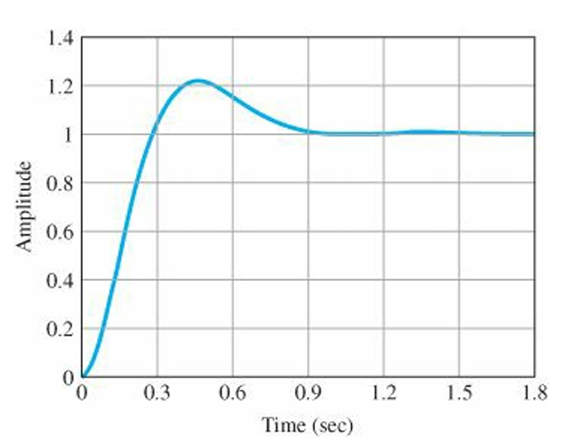
Find a compensation for $G(s) = \frac{1}{s(s+1)}$ that will provide overshoot of no more than 20% and rise time of no more than 0.3 sec.
Note that $M_p$(overshoot) is the maximum amount of the overshoot divided by the final value where $M_p=y(t_p)-1=e^{-\sigma\pi/\omega_d}=e^{-\pi\zeta/\sqrt{1-\zeta^2}}$ and $t_r$(rise time) is the time to reach the vicinity of the new set point where $t_r\approx \frac{1.8}{\omega_n}$
So, the requirement is $\zeta\geq 0.5$ and $\omega_n\cong \frac{1.8}{0.3}=6$.
To provide some margin, we'll shoot for $\zeta\geq 0.5$ and $\omega_n\geq 7 rad/sec$.
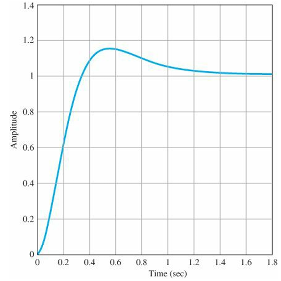
But the step response of the system exceeds the overshoot specification a small amount.
Typically, lead compensation in the feed forward path will increase the step-response overshoot because the zero of the compensation has a differentiating effect.
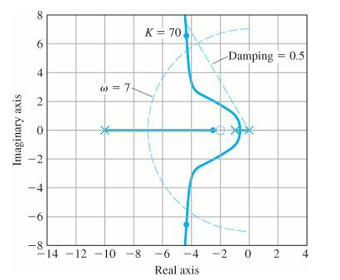
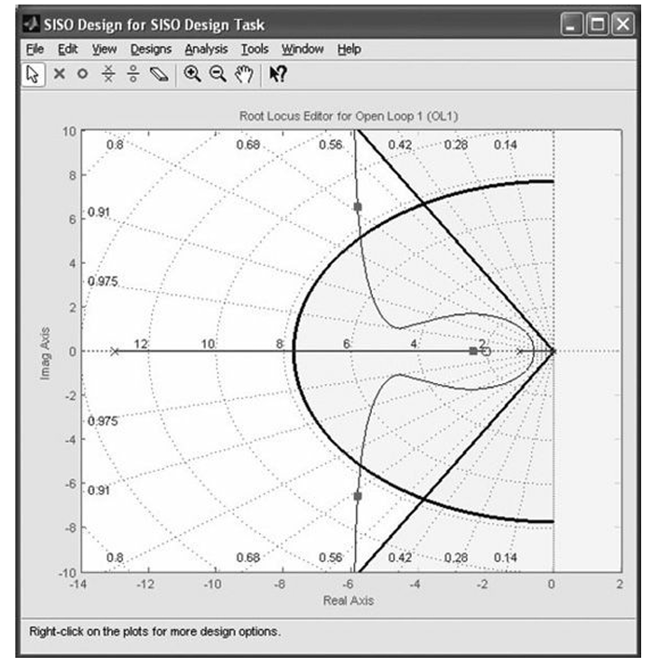
We can tune the compensator to achieve better damping in order to reduce the overshoot in the transient response using RLTOOL.
By moving the pole of the lead compensator more to the left in order to pull the locus in that direction, andselecting K = 91, we obtain $$D(s)=91\frac{s+2}{s+13}$$
The phase at $s=j\omega$ is given by $$\phi=\tan^{-1}\left ( \frac{\omega}{z} \right )-\tan^{-1}\left ( \frac{\omega}{p} \right )$$
If $z < p$, then $\phi$ is positive, which by definition indicates phase lead.
Lag Compensation
Once satisfactory dynamic response has been obtained, perhaps by using one or more lead compensations, we may discover that the low-frequency gain—the value of the relevant steady-state error constant, such as $K_v$—is still too low.
The system type, which determines the degree of the polynomial the system is capable of following, is determined by the order of the pole of the transfer function $D(s)G(s)$ at $s = 0$. If the system is Type 1, the velocity-error constant, which determines the magnitude of the error to a ramp input, is given by $\displaystyle \lim_{s \to 0}sG(s)D(s)$.
In order to increase this constant, it is necessary to do so in a way that does not upset the already satisfactory dynamic response. Thus, we want an expression for $D(s)$ that will yield a significant gain at s = 0 to raise $K_v$ (or some other steady-state error constant) but is nearly unity (no effect) at the higher frequency $\omega_n$, where dynamic response is determined. The solution is lag compensation. $$D(s)=\frac{s+z}{s+p},\quad z>p$$
The values of z and p are small compared with $\omega_n$, yet $D(0) = \frac{Z}{p} = 3\;to\;10$ (the value depending on the extent to which the steady-state gain requires boosting) Because z > p, the phase $\phi$ is negative, corresponding to phase lag.
e.g.
Consider $$G(s)=\frac{1}{s(s+1)}$$
with lead compensator $$KD_1(s)=K\frac{s+2}{s+13}$$
with the gain of $K=91$ from the previous example, the velocity constant is $$K_v=\displaystyle \lim_{s \to 0}sKD_1G=\displaystyle \lim_{s \to 0}s(91)\frac{s+2}{s+13}\frac{1}{s(s+1)}=\frac{91*2}{13}=14$$
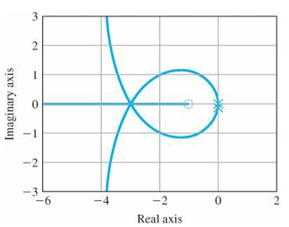
Suppose we require that $K_v = 70$. To obtain this, we require a lag compensation with $Z/p = 5$ in order to increase the velocity constant by a factor of 5. This can be accomplished with a pole at $p= -0.01$ and a zero at $z = -0.05$, which keeps the values of both z and p very small so that $D_2(s)$ would have little effect on the portions of the locus representing the dominant dynamics around $\omega_n=7$. The lag compensation transfer function is $$D_2(s)=\frac{s+0.05}{s+0.01}$$
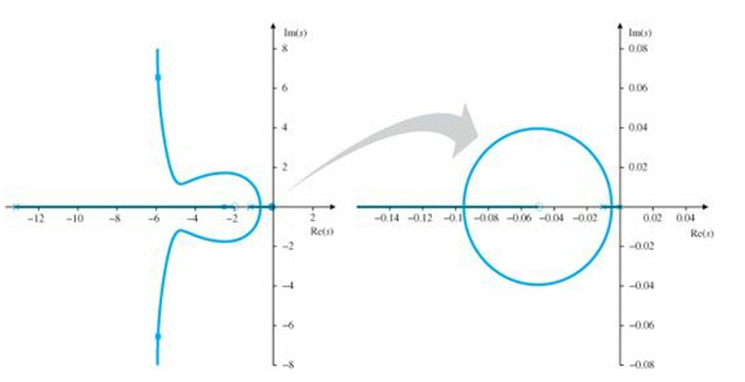
$$KD(s)=91\frac{s+2}{s+13}\frac{s+0.05}{s+0.01}$$
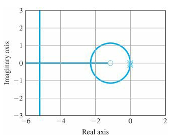
With $K = 91$, the dominant roots are at $-5.8 \pm j6.5$. The effect of the lag compensation can be seen by expanding the region of the locus around the origin(right side of the figure above). The circular locus is a result of the small pole and zero. The transient response corresponding to this root will be a very slowly decaying term, which will have a small magnitude because the zero will almost cancel the pole in the transfer function. The decay is so slow that this term may seriously influence the settling time, and zero will not be present in the step response to a disturbance torque and the slow transient will be much more evident there. That's why it is important to place the lag pole-zero combination at as high a frequency as possible without causing major shifts in the dominant root locations.
Notch Compensation
The lead and lag compensation above is found to have a substantial oscillation at about 50 rad/sec when tested, because there was an unsuspected flexibility of the noncollocated type at a natural frequency of $\omega_n=50$. On reexamination, the plant transfer function, including the effect of the flexibility, is estimated to be $$G(s)=\frac{2500}{s(s+1)(s^2+s+2500)}$$
the very lightly damped roots at 50 rad/sec have been made even less damped or perhaps unstable by the feedback. The best method to fix this situation is to modify the structure so that there is a mechanical increase in damping. Unfortunately, this is often not possible because it is found too late in the design cycle.
How to correct this oscillation?
approach 1) Gain Stabilization: reducing the gain at high frequency
add lag compensation
it might lower the loop gain far enough that there is greatly reduced spillover and the oscillation is eliminated.
approach 2) Phase Stabilization
add a zero near the resonance
this approach can be used if the response time resulting from gain stabilization is too long.
it shifts the departure angles from the resonant poles so as to cause the closed-loop root to move into the LHP, thus causing the associated transient to die out. the result is called a notch compensation which has a transfer function of $$D_{notch}(s)=\frac{s^2+2\zeta\omega_0s+\omega_0^2}{(s+\omega_0)^2}$$
A necessary design decision is whether to place the notch frequency above or below that of the natural resonance of the flexibility in order to get the necessary phase. A check of the angle of departure shows that with the plant compensated and the notch as given, it is necessary to place the frequency of the notch above that of the resonance to get the departure angle to point toward the LHP. Thus the compensation is added with the transfer function $$D_{notch}(s)=\frac{s^2+0.8s+3600}{(s+60)^2}$$
When considering notch or phase stabilization, it is important to understand that its success depends on maintaining the correct phase at the frequencyofthe resonance. If that frequency is subject to significant change, which is common in many cases, then the notch needs to be removed far enough from the nominal frequency in order to work for all cases. The result may be interference of the notch with the rest of the dynamics and poor performance. As a general rule, gain stabilization is substantially more robust to plant changes than is phase stabilization.
it can determine the natural frequency (constant term in eqn)
it can't determine the damping
system type 0
if $k_p$ is made large to get adequately small steady-state error, the damping may be much too low for satisfactory transient response with proportional control alone.
Proportional Plus Integral Control (PI)
Add an integral term to the controller to get the automatic reset effect results in the proportional plus integral control equation in the time domain.
$$u(t)=k_pe+k_I\int_{t_0}^{t}e(\tau)d\tau$$
$$\frac{U(s)}{E(s)}=D_{cl}(s)=k_p+\frac{k_I}{s}$$
system type 1
reject completely constant bias disturbances
e.g.
plant: $$Y=\frac{A}{\tau s+1}(U+W)$$
transform eqn for controller: $$U=k_p(R-Y)+k_I\frac{R-Y}{s}$$
Step response of process control system: process reaction curve as below:
Process Reaction Curve
$$\frac{Y(s)}{U(s)}=\frac{Ae^{-st_d}}{\tau s+1}$$
1. Tuning by decay ratio of 0.25
desigining goal: closed-loop step response transient with a decay ratio of approximately 0.25 (corresponding to $\zeta=0.21$)
2. Tuning by evaluation at limit of stability (ultimate sensitivity method)
Criteria for adjusting the parameters are based on evaluating the amplitude and frequency of the oscillations of the system at the limit of stability
The proportional gain is increased until the system becomes marginally stable and continuous oscillations just begin with amplitude limited by the saturation of the actuator. The corresponding gain is defined as $K_u$ (called the ultimate gain) and the period of oscillation is $P_u$ (called the ultimate period).
$P_u$ should be measured when the amplitude of oscillation is as small as possible.
$$D_c(s)=k_p(1+\frac{1}{T_Is}+T_Ds)$$
Determination of ultimate gain and periodNeutrally stable system
This category is based on 'Feedback Control of Dynamic System 6th edition' (Franklin).
Outline of the book:
Ch.1 the essential ideas of feedback and some of the key design issues, history of control
Ch.2 dynamic modeling with mechanical, electrical, electromechanical, fluid, and thermodynamic devices
Ch.3 dynamic response, correlation between pole locations and transient response, the effects of extra zeros and poles on dynamic response, stability of dynamic system
Ch.4 basic equations and transfer functions of feedback along with the definitions of the sensitivity function, open-loop and closed-loop control, PID Control Structure
Ch.5 design methods based on root locus
Ch.6 design methods based on frequency response
Ch.7design methods based on state-variable feedback
Ch.8 design feedback control for implementation in a digital computer