feedback control system을 디자인하는 여러 방법 중 하나인 State-Space method를 다루도록 한다.
State-Space Design은 시스템의 state-variable을 직접 다루며 동적 보상을 설계하는 과정이다. 즉, 주어진 환경에서 목표로 하는 design specifications에 맞는 compensation $D(s)$를 찾는 것이 State-Space method의 역할이다.

The steps of the design method
1. Select closed-loop pole (root as referred to in previous chapters) locations and develop the control law for the closed-loop system that corresponds to satisfactory dynamic response
2. Design an estimator
3. Combine the control law and the estimator
4. Introduce the reference input
Advantages of State-Space
The differential equations describing a dynamic system are organized as a set of first-order differential equations in the vector-valued state of the system, and the solution is visualized as a trajectory of this state vector in space. ODEs of physical dynamic systems can be manipulated into state-variable form. In the field of Normal form mathematics, where ODEs are studied, the state-variable form is called the normal form for the equations.
System Description in State-Space
$$\dot{\textbf{x}}=\textbf{Fx}+\textbf{G}u\quad where\quad y=\textbf{Hx}+Ju$$
$F: n \times n, G: n \times 1, H: 1 \times n, J: scalar$
ex 7.1)
Dynamics: $$I\ddot{\theta}=F_cd+M_D$$
다음 위성 자세 제어 모델을 state-variable form으로 표현하자. 이때 input은 $u=F_c$이고 $M_D=0$을 가정한다.
$$\dot{\theta}=\omega,\quad\dot{\omega}=\frac{d}{I}F_c$$

$$\frac{\mathrm{d} }{\mathrm{d} t} \begin{bmatrix}
\theta \\\omega
\end{bmatrix}\begin{bmatrix}
0& 1\\
0& 0\\
\end{bmatrix}\begin{bmatrix}
\theta \\\omega
\end{bmatrix} +\begin{bmatrix}
0 \\d/I
\end{bmatrix}F_c$$
시스템의 output은 위성의 자세($y=\theta$)이므로,
$$y=\begin{bmatrix}
1 & 0 \\
\end{bmatrix}\begin{bmatrix}
\theta \\ \omega
\end{bmatrix}+0\cdot u$$
따라서 state-variable form에 대한 행렬은 다음과 같다.
$$\textbf{F}=\begin{bmatrix}
0 &1 \\
0 &0 \\
\end{bmatrix},\quad \textbf{G}=\begin{bmatrix}
0 \\ d/I
\end{bmatrix},\quad \textbf{H} = \begin{bmatrix}
1 &0 \\
\end{bmatrix},\quad J=0$$
ex 7.2)
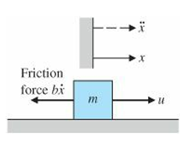
Dynamics: $$ \ddot{x}+\frac{b}{m}\dot{x}=\frac{u}{m}$$
$$\dot{x}=v,\quad\dot{v}=-\frac{b}{m}v+\frac{1}{m}u$$
$$\frac{\mathrm{d} }{\mathrm{d} t} \begin{bmatrix}
x\\v
\end{bmatrix}=\begin{bmatrix}
0 &1 \\
0 &-b/m \\
\end{bmatrix}\begin{bmatrix}
x \\v
\end{bmatrix}+\begin{bmatrix}
0 \\1/m
\end{bmatrix}u$$
a) 시스템의 output을 position $y=x_1=x$로 정하자.
$$y=\begin{bmatrix}
1 &0 \\
\end{bmatrix}\begin{bmatrix}
x \\v
\end{bmatrix}$$
따라서 state-variable form에 대한 행렬은 다음과 같다.
$$\textbf{F}=\begin{bmatrix}
0 &1 \\
0 &-b/m \\
\end{bmatrix},\quad \textbf{G}=\begin{bmatrix}
0 \\1/m
\end{bmatrix},\quad \textbf{H}= \begin{bmatrix}
1 &0 \\
\end{bmatrix}, J=0$$
b) 시스템의 output을 velocity $v=x_2$로 정하자.
다른 행렬은 동일하고 output matrix H만 달라지게 된다.
$$H=\begin{bmatrix}
0 &1 \\
\end{bmatrix}$$
Step Response를 다음처럼 얻을 수 있다.
% MATLAB CODE %
F=[0 1;0 –0.05];
G=[0;0.001]; H=[0 1];
J = 0;
sys = ss(F, 500*G,H,J); % step gives unit step response, so 500*G gives u = 500 N.
step(sys); % plots the step response
Block Diagrams and State-Space
ex 7.7)
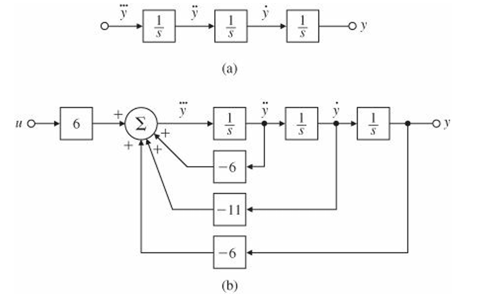
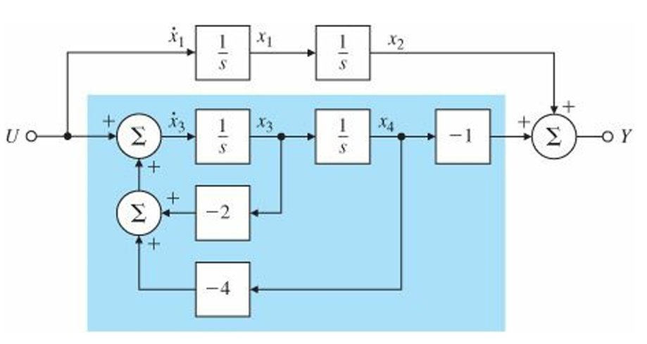
Let's find a state-variable description and the transfer function of the third-order system whose differential eqn is $$\dddot{y}+6\ddot{y}+11\dot{y}+6y=6u$$
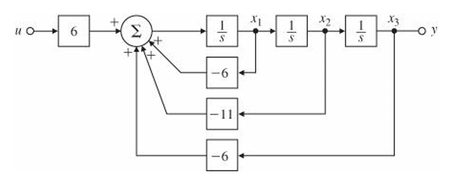
$$x_1=\ddot{y},\;x_2=\dot{y},\;x_3=y$$
$$\dot{x}_1=-6x_1-11x_2-6x_3+6u$$
$$\dot{x}_2=x_1$$
$$\dot{x}_3=x_2$$
$$\textbf{F}=\begin{bmatrix}
-6 &-11 &-6 \\
1 &0 &0 \\
0 &1 &0 \\
\end{bmatrix},\quad \textbf{G}=\begin{bmatrix}
6 \\0\\0
\end{bmatrix},\quad \textbf{H}= \begin{bmatrix}
0 &0 &1 \\
\end{bmatrix}, J=0$$
% yield the transfer function
[num,den] =ss2tf(F,G,H,J);

% convert state-variable realization to pole-zero form
[z,p,k] =ss2zp(F,G,H,J)

% convert numerator-denominator to pole-zero form
[z,p,k] =tf2zp(num,den)
$$\frac{Y(s)}{U(s)}=\frac{6}{s^3+6s^2+11s+6}=\frac{6}{(s+1)(s+2)(s+3)}$$
Time and Amplitude Scaling in State-Space
Time scaling with $\tau=\omega_0t$:
$$\frac{\mathrm{d} \textbf{x}}{\mathrm{d} \tau}=\frac{1}{\omega_0}\textbf{Fx}+\frac{1}{\omega_0}\textbf{G}u=\textbf{F}'\textbf{x}+\textbf{G}'u$$
Amplitude scaling:
replacing $x$ with $\textbf{z}=\textbf{D}_x^{-1} \textbf{x}$ where $\textbf{D}_x$ is a diagonal matrix of scale factors
replacing $u$ with $v=\textbf{D}_u^{-1}u$
$$\textbf{D}_x\dot{\textbf{z}}=\frac{1}{\omega_0}\textbf{F}\textbf{D}_x\textbf{z}+\frac{1}{\omega_0}\textbf{G}\textbf{D}_uv$$
Then $$\dot{\textbf{z}}=\frac{1}{\omega_0}\textbf{D}_x^{-1}\textbf{F}\textbf{D}_x\textbf{z}+\frac{1}{\omega_0}\textbf{D}_x^{-1}\textbf{G}\textbf{D}_uv=\textbf{F}'\textbf{z}+\textbf{G}'v$$
Block Diagrams and Canonical Forms
다음 전달 함수를 갖는 시스템을 생각하자.
$$G(s)=\frac{b(s)}{a(s)}=\frac{s+2}{s^2+7s+12}=\frac{2}{s+4}+\frac{-1}{s+3}$$
Control Canonical Form
$$\dot{\textbf{x}}=\textbf{A}_c\textbf{x}+\textbf{B}_cu,\quad y=\textbf{C}_c\textbf{x}$$
$b(s)$의 근은 전달 함수의 zeros이고, $a(s)$의 근은 전달 함수의 poles이다.

block diagram으로부터 다음 관계식을 얻을 수 있다.
$$\dot{x}_1=-7x_1-12x_2+u,\quad\dot{x}_2=x_1\quad y=x_1+2x_2$$
이로부터 control canonical form의 matrix를 구할 수 있다.
$$\textbf{A}_c=\begin{bmatrix}
-7 &-12 \\
1 &0 \\
\end{bmatrix},\quad
\textbf{B}_c=\begin{bmatrix}
1 \\0
\end{bmatrix},\quad
\textbf{C}_c=\begin{bmatrix}
1 &2 \\
\end{bmatrix},\quad
D_c=0$$
$b(s)$의 계수인 1, 2가 $\textbf{C}_c$ 행렬에 나타나고, $a(s)$에서 최고차항을 제외한 계수 7, 12가 $\textbf{A}_c$의 1열에 반대 부호로 나타난다.
따라서, 다음 전달 함수에 대한 Control Canonical Form은 아래와 같이 결정된다.
$$\frac{b(s)}{a(s)}=\frac{b_1s^{n-1}+b_2s^{n-2}+\cdots b_n}{s^n+a_1s^{n-1}+a_2s^{n-2}+\cdots a_n}$$
$$\textbf{A}_c=\begin{bmatrix}
-a_1 &-a_2 &\cdots &\cdots &-a_n \\
1 &0 &\cdots &\cdots &0 \\
0 &1 &\cdots &\cdots &0 \\
\vdots & &\ddots &\vdots &\vdots \\
0 &\cdots &\cdots &1 &0 \\
\end{bmatrix},\quad
\textbf{B}_c=\begin{bmatrix}
1 \\0 \\ \vdots \\ 0
\end{bmatrix},$$
$$\textbf{C}_c=\begin{bmatrix}
b_1 &b_2 &\cdots &b_n \\
\end{bmatrix},\quad
D_c=0$$
num = b = [b1 b2 ... bn ]
den = a = [1 a2 ... an]
[Ac, Bc, Cc, Dc] =tf2ss(num,den).
Modal Canonical Form
$$\dot{\textbf{z}}=\textbf{A}_m\textbf{z}+\textbf{B}_mu,\quad y=\textbf{C}_m\textbf{z}+D_mu$$
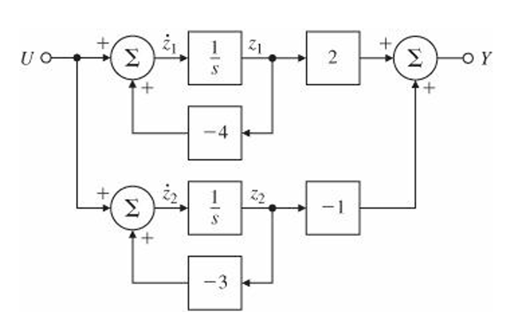
$$\textbf{A}_m=\begin{bmatrix}
-4 &0 \\
0 &-3 \\
\end{bmatrix},\quad
\textbf{B}_m=\begin{bmatrix}
1 \\1
\end{bmatrix},\quad
\textbf{C}_m=\begin{bmatrix}
2 &-1 \\
\end{bmatrix},\quad
D_m=0$$
전달함수가 분수의 합으로 표현된 부분을 살펴보면 poles(-4, -3)이 $\textbf{A}_m$ 행렬의 대각선에 들어가 있고, 각 분수의 분자(2, -1)이 $\textbf{C}_m$에 나타난다.
canonical form으로 나타낼 때 맞닥뜨릴 수 있는 어려움이 두 가지 있다.
1) the elements of the matrices will be complex when the poles of the system are complex
express the complex poles of the partial-fraction expansion as conjugate pairs in second-order terms so that all the elements remain real. The corresponding $\textbf{A}_m$ matrix will then have 2 × 2 blocks along the main diagonal representing the local coupling between the variables of the complex-pole set.
2) the system matrix cannot be diagonal when the partial-fraction expansion has repeated poles
couple the corresponding state-variables, so that the poles appear along the diagonal with off-diagonal terms indicating the coupling.
ex) $G(s)=1/s^2$
$$\textbf{F}=\begin{bmatrix}
0 &1 \\
0 &0 \\
\end{bmatrix},\quad
\textbf{G}=\begin{bmatrix}
0 \\1
\end{bmatrix},\quad
\textbf{H}=\begin{bmatrix}
1 &0 \\
\end{bmatrix},\quad
J=0$$
ex 7.9)
다음 전달 함수에 대한 modal form의 state matrices를 찾아보자
$$G(s)=\frac{2s+4}{s^2(s^2+2s+4)}=\frac{1}{s^2}-\frac{1}{s^2+2s+4}$$
$$\textbf{F}=\begin{bmatrix}
0&0&0&0 \\
1&0&0&0 \\
0&0&-2&-4\\
0&0&1&0\\
\end{bmatrix},\quad
\textbf{G}=\begin{bmatrix}
1\\0\\1\\0
\end{bmatrix},\quad$$
$$\textbf{H}=\begin{bmatrix}
0&1 &0&-1 \\
\end{bmatrix},\quad
J=0$$
'Study > Control' 카테고리의 다른 글
| Observability (0) | 2025.01.30 |
|---|---|
| Controllability (0) | 2025.01.30 |
| Frequency-Response Design (0) | 2025.01.15 |
| Root Locus, Compensation (0) | 2025.01.13 |
| PID Control (1) | 2025.01.04 |