산업에서 Feedback Control System을 디자인할 때 Frequency-Response를 많이 활용한다고 한다. 특히 Plant model의 불확실성 면에서 좋은 디자인을 제공해줄 수 있다.
사인파 입력(sinusoidal inputs)에 대한 선형 시스템의 response를 그 시스템의 Frequency Response라 한다. 이는 pole and zero locations으로부터 알 수 있다.
we consider a system described by $$\frac{Y(s)}{U(s)}=G(s)$$ where the input $u(t)$ is a sine wave with an amplitude $A$: $$u(t)=A\sin(\omega_0t)1(t)$$
$u(t)$를 라플라스 변환하면 $U(s)=\frac{A\omega_0}{s^2+\omega_0^2}$이므로, $$Y(s)=G(s)\frac{A\omega_0}{s^2+\omega_0^2}$$
$Y(s)$를 Partial Expansion 하자. (일단 $G(s)$의 poles이 모두 distinct라 가정)
$$Y(s)=\frac{\alpha_1}{s-p_1}+\frac{\alpha_2}{s-p_2}+\cdots+\frac{\alpha_n}{s-p_n}+\frac{\alpha_0}{s+j\omega_0}+\frac{\alpha_0^*}{s-j\omega_0}$$
$$y(t)=\alpha_1e^{p_1t}+\alpha_2e^{p_2t}+\cdots+\alpha_ne^{p_nt}+2\left |\alpha_0 \right |\cos(\omega_0t+\phi),\quad t\geq0$$ where $$\phi=tan^{-1}\left [ \frac{Im(\alpha_0)}{Re(\alpha_0)} \right ]$$
If all the poles of the system represent stable behavior (the real parts of $p_1, p_2, . . . , p_n < 0$), the natural unforced response will die out eventually, and therefore the steady-state response of the system will be due solely to the sinusoidal term.
Using cover-up method, $$\alpha_0=(s+j\omega_0)Y(s)|_{s=-j\omega_0}=G(-j\omega_0)\frac{A\omega_0}{-2j\omega_0}=-\frac{A}{2j}G(-j\omega_0)$$
$$\alpha_0^*=(s-j\omega_0)Y(s)|_{s=j\omega_0}=G(j\omega_0)\frac{A\omega_0}{2j\omega_0}=\frac{A}{2j}G(j\omega_0)$$
$$\displaystyle \lim_{t \to 0}y(t)\approx \alpha_0e^{-j\omega_0t}+\alpha_0^*e^{j\omega_0t}=A\left | G(j\omega_0)\right |\frac{-e^{j(\omega_0t+\phi)}+e^{j(\omega_0t+\phi)}}{2j}=A\left | G(j\omega_0)\right |\sin(\omega_0t+\phi)=AM\sin(\omega_0t+\phi)$$
where $$M=\left | G(j\omega_0)\right |=\left | G(s)\right ||_{s=j\omega_0}=\sqrt{\left\{Re[G(j\omega_0)]\right\}^2+\left\{Im[G(j\omega_0)]\right\}^2}$$
$$\phi=\tan^{-1}\left[\frac{Im[G(j\omega_0)]}{Re[G(j\omega_0)]}\right]=\angle G(j\omega_0)$$
Magnitude와 phase를 각각 frequency에 대하여 표현함으로써 시스템의 특성을 확인할 수 있다.
극형식으로부터 $G(j\omega_0)=Me^{j\phi}$로 표현할 수 있다.
ex 6.2)
예시를 통해 lead compensator의 Frequency-Response 특성을 알아보자.
lead compensator with $$D(s)=K\frac{Ts+1}{\alpha Ts+1},\quad\alpha<1$$
$$D(j\omega)= K\frac{Tj\omega+1}{\alpha Tj\omega+1}$$
$$M=\left|D\right|= \left | K\right |\frac{\sqrt{1+(\omega T)^2}}{\sqrt{1+(\alpha\omega T)^2}}$$
$$\phi=\angle(1+j\omega T)-\angle(1+j\alpha\omega T)=tan^{-1}(\omega T)-tan^{-1}(\alpha\omega T)$$
MATLAB으로 $D(j\omega)$를 그려보자. $(K = 1, T = 1, \;and\; α = 0.1 \;for\; 0.1 ≤ ω ≤ 100)$
num = [1 1];
den = [0.1 1];
sysD = tf(num, den);
w = logspace(-1, 2);

[mag, phase] = bode(sysD, w);

loglog(w, squeeze(mag)), grid;
semilogx(w, squeeze(phase)), grid;
Magnitude는 low frequency일 때 $1(=K)$, high frequency일 때 $10(=K/\alpha)$인 것을 확인할 수 있다. Phase는 low and high frequency일 때 phase가 0에 가까워지고 중간 즈음의 frequency에서 높은 phase가 나타나는 것을 관찰할 수 있다.
Transfer Function에 대하여 frequency에 따른 Magnitude와 Phase는 시스템의 dynamic response에 대한 정보를 제공한다. sinusoid input에 대하여 $M$과 $\phi$는 response를 온전히 묘사할 수 있고, periodic input의 경우 푸리에 급수를 통해 sum of sinusoids로 분해하여 total response를 분석할 수 있다. transient input에 대하여는 $G(j\omega)$와 라플라스 변환을 통해 얻은 transient response 간의 관계를 통해 이해하는 것이 좋다.
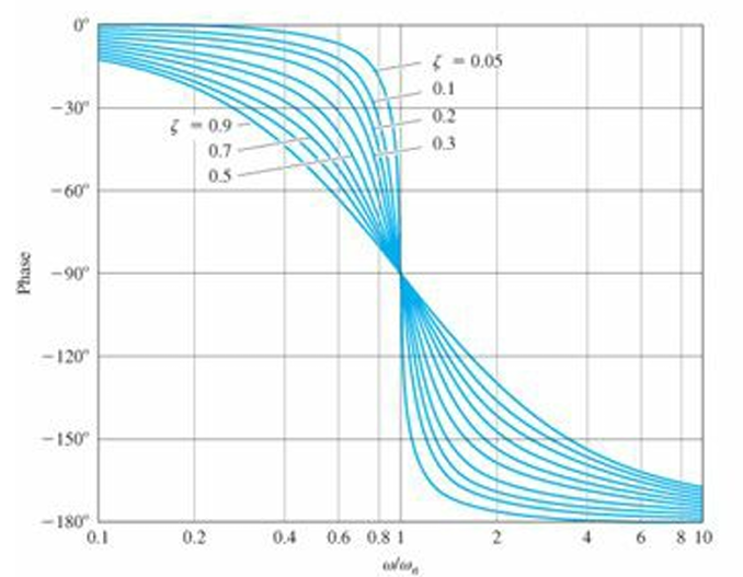
다음 전달함수를 생각해 보자. $$G(s)=\frac{1}{(s/\omega_n)^2+2\zeta(s/\omega_n)+1}$$
$\zeta$ 값에 따른 $M(\omega)$와 $\phi(\omega)$의 분포는 다음과 같다. 시스템의 damping이 transient response overshoot나 magnitude peak에 영향을 미치는 것을 관찰할 수 있다. 또한 $\omega_n$이 거의 bandwidth와 비슷하므로 bandwidth로부터 rise time을 추정할 수 있다. $\zeta<0.5$에서 peak overshoot이 약 $1/2\zeta$인 것도 확인할 수 있다.

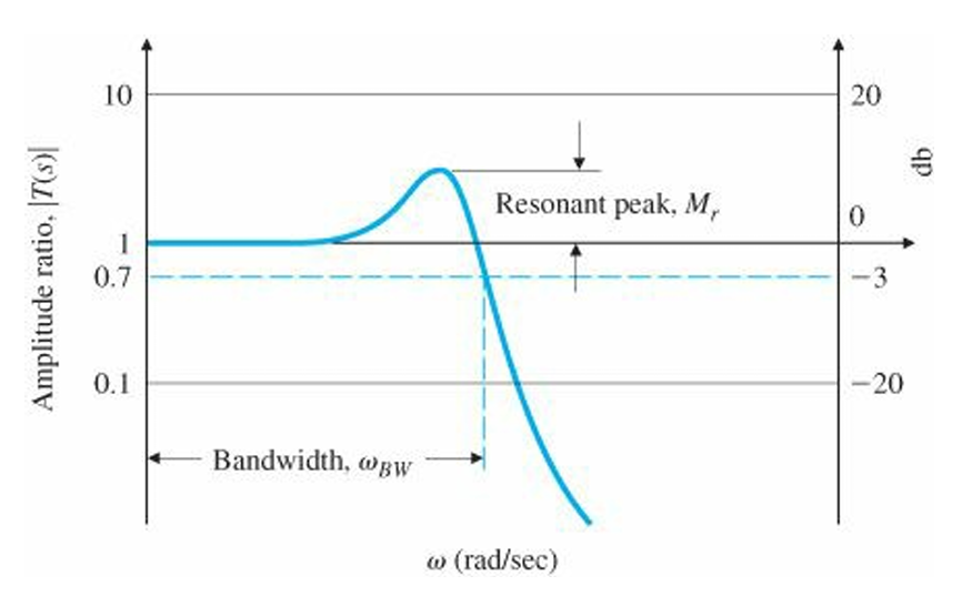
Bandwidth
A natural specification for system performance in terms of frequency response is the bandwidth, defined to be the maximum frequency at which the output of a system will track an input sinusoid in a satisfactory manner. By convention, for the system with a sinusoidal input $r$, the bandwidth is the frequency of $r$ at which the output $y$ is attenuated to a factor of 0.707 times the input. $$\frac{Y(s)}{R(s)}\overset{\underset{\mathrm{def}}{}}{=}T(s)=\frac{KG(s)}{1+KG(s)}$$
Bandwidth is a measure of speed of response and is therefore similar to time-domain measures such as rise time and peak time or the s-plane measure of dominant-root(s) natural frequency. In fact, if the $KG(s)$ is such that the closed-loop response is given by the graphs above, we can see that the bandwidth will equal the natural frequency of the closed-loop root (that is, $\omega_{BW} = \omega_n$ for a closed-loop damping ratio of $\zeta = 0.7$). For other damping ratios, the bandwidth is approximately equal to the natural frequency of the closed-loop roots, with an error typically less than a factor of 2.

Bandwidth의 정의는 physical control system 등 low-pass filter behavior가 있는 시스템에 대하여 논할 때 의미가 있다. 그 외의 적용에 있어 Bandwidth는 다소 다르게 정의될 수 있다. 또한 high-frequency roll-off, 즉 고주파에서 값이 떨어지는 현상이 일어나지 않는 이상적인 시스템이라면 bandwidth는 무한대가 된다(e.g. # of poles = # of zeros).
Bode Plot
Magnitude curve는 log scale로, Phase curve는 linear scale로 그려 high-order system을 그릴 수 있다.
$$G(j\omega)=Me^{j\phi}=\frac{r_1e^{j\theta_1}r_2e^{j\theta_2}}{r_3e^{j\theta_3}r_4e^{j\theta_4}r_5e^{j\theta_5}}$$라 하자. 그러면 $$\left |G(j\omega) \right |=\frac{r_1r_2}{r_3r_4r_5},$$
where $$\log_{10}M=\log_{10}r_1+\log_{10}r_2-\log_{10}r_3-\log_{10}r_4-\log_{10}r_5$$
$$\phi=\theta_1+\theta_2-\theta_3-\theta_4-\theta_5$$
$$\log_{10}Me^{j\phi}=\log_{10}M+j\phi\log_{10}e$$
Decibel (db)
통신에서는 power gain을 decibel로 측정하는 것이 표준이다.
Power $P$, Voltage $V$에 대해서, $$\left |G \right |_{db}=10\log_{10}\frac{P_2}{P_1}=20\log_{10}\frac{V_2}{V_1}$$
따라서 Bode plot을 $\left |G \right |_{db}$ vs. $\log \omega$와 Phase (deg) vs. $\log \omega$ 로 표현할 수 있다. 이때 Magnitude에서 log를 씌워서 수직 방향 스케일이 db과 선형적이도록 표현하곤 한다.
Advantages of Bode plots
1. Dynamic compensator design can be based entirely on Bode plots.
2. Bode plots can be determined experimentally.
3. Bode plots of systems in series (or tandem) simply add, which is quite convenient.
4. The use of a log scale permits a much wider range of frequencies to be displayed on a single plot than is possible with linear scales.
Classes of terms of transfer functions
앞에서 다룬 여러 전달함수에서의 terms을 크게 세 가지로 분류하였다.
Class 1. $K_0(j\omega)^n$
*singularities at the origin
$$\log K_0\left | (j\omega)^n\right |=\log K_0+n\log\left | j\omega\right |$$
Magnitude Plot 기울기가 n x (20 db per decade)인 직선으로 그려지게 된다.

Class 2. $(j\omega\tau+1)^{\pm1}$
*first-order term
Magnitude Plot은 낮은 주파수일 때와 높은 주파수일 때 각각 다른 점근선(Asymptotes)을 갖는다.
For $\omega\tau\ll 1$, $j\omega\tau+1\cong 1$
For $\omega\tau\gg 1$, $j\omega\tau+1\cong j\omega\tau$
$\omega=1/\tau$를 break point라 칭한다. break point보다 작은 주파수에서는 magnitude가 거의 상수고 break point보다 큰 주파수에서는 Class 1과 유사한 양상을 보인다.
아래의 그림은 $\tau=10$일 때, 즉 $G(s)=10s+1$일 때의 magnitude plot이다. break point에서 점근선과 실제 곡선의 차이가 1.4 정도 (3 db) 있는 것을 관찰할 수 있다. break point 이전의 주파수에서는 거의 0 db이고, break point 이후의 주파수에서는 기울기가 +1(or +20 db per decade)이다.

Phase는 주파수의 범위에 따라 점근선을 크게 세 개로 나눌 수 있다.
For $\omega\tau\ll 1$, $\angle 1=0^\circ$
For $\omega\tau\gg 1$, $\angle j\omega\tau=90^\circ$
For $\omega\tau\cong1$, $\angle (j\omega\tau+1)=45^\circ$

Class 3. $\left [ \frac{j\omega}{\omega_n}+2\zeta\frac{j\omega}{\omega_n}+1 \right ]^{\pm1}$
*second-order term
break point는 $\omega=\omega_n$으로 한다.
큰 양상은 Class 2와 유사하다. Magnitude는 break point로부터 기울기 +2(or +40 db per decade)를 갖는 직선 형태다. second-order term이 분모에 있다면 기울기는 -2다. Phase도 마찬가지로 Class 2의 두 배인 $\pm 180^{\circ}$로 변화한다.
다만 damping ratio $\zeta$에 따라 break point 주변의 transition이 다르다. 위의 Figure 6.3에서 그 모습을 확인할 수 있다.
Peak Amplitude: Figure 6.3과 같이 second-order term이 분모에 있는 경우 Magnitude의 최댓값은 break point에서 발생하며 그 값은 $\left | G(j\omega_n)\right |=1/2\zeta$ 이다.
break point에서의 Phase는 $\angle=G(j\omega_n)=\pm90^\circ$이다.
Composite Curve
poles과 zeros가 여러 개 있는 시스템의 경우 frequency response는 각 component가 결합된 composite curve로 표현된다. Composite Magnitude Curve는 각 curve 점근선의 기울기를 합한 것이고, Composite Phase Curve는 각 curve를 그대로 합한 것이다. 이 규칙은 우선 LHP의 poles과 zeros에 대한 것이며 changes for singularities in RHP는 추후 고려하도록 한다.
ex 6.3)
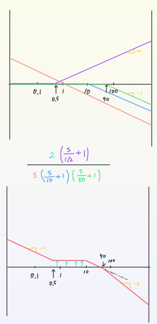
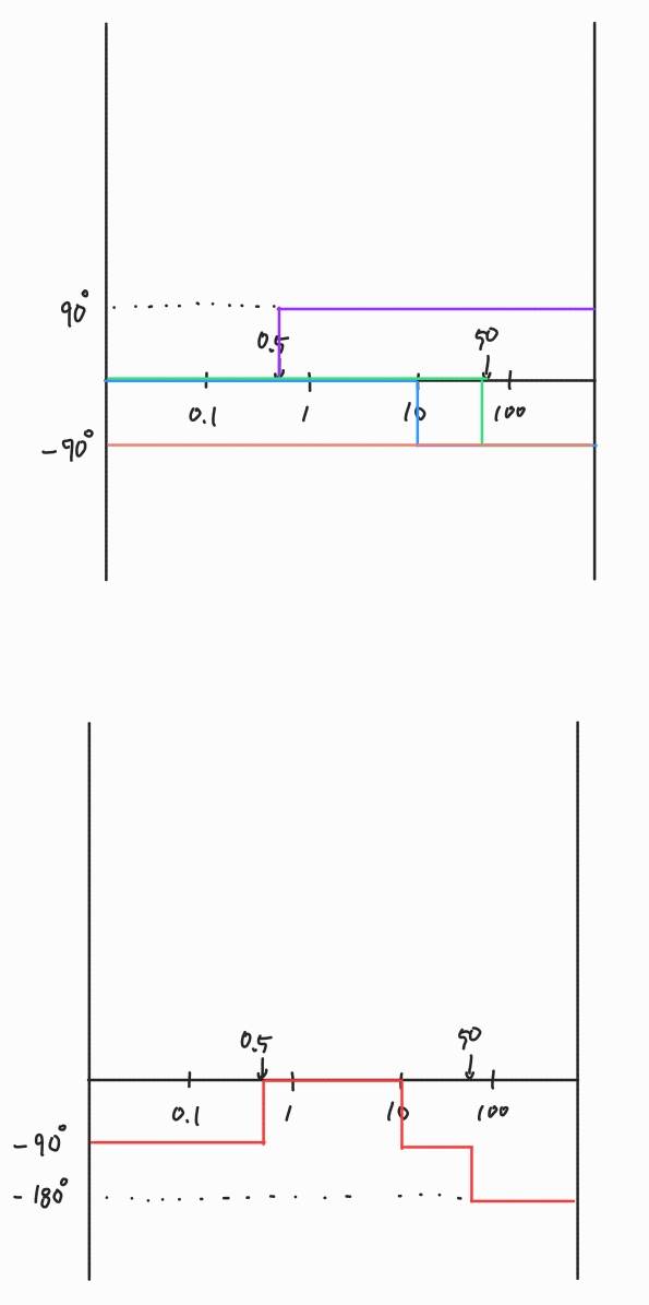
다음 전달 함수의 Bode Plot을 그려보자. $$KG(s)=\frac{2000(s+0.5)}{s(s+10)(s+50)}$$
먼저 각 term을 Class 1~3의 형태로 바꾸어 계산을 용이하게 한다.
$$KG(s)=\frac{2000\cdot \frac{1}{2}(\frac{s}{1/2}+1)}{500s(\frac{s}{10}+1)(\frac{s}{50}+1)}=\frac{2(\frac{s}{1/2}+1)}{s(\frac{s}{10}+1)(\frac{s}{50}+1)}$$
그리고 $s=j\omega$를 대입한다. $$KG(j\omega)=\frac{2(\frac{j\omega}{0.5}+1)}{j\omega(\frac{j\omega}{10}+1)(\frac{j\omega}{50}+1)}$$
각 term으로 인한 점근선을 그린 후 합성하여 Magnitude 및 Phase의 점근선을 나타낼 수 있다. 빨간색 점근선을 따라 그래프가 그려지게 될 것이다.


'Study > Control' 카테고리의 다른 글
| Controllability (0) | 2025.01.30 |
|---|---|
| State-Space Design (0) | 2025.01.30 |
| Root Locus, Compensation (0) | 2025.01.13 |
| PID Control (1) | 2025.01.04 |
| Laplace Transform & Transfer Function (0) | 2025.01.04 |