
For this system, the closed-loop transfer function is $$\frac{Y(s)}{R(s)}=\frac{D(s)G(s)}{1+D(s)G(s)H(s)}$$ and the characteristic eqn, whose roots are the poles of this transfer function, is $$1+D(s)G(s)H(s)=0$$
Let the open loop transfer function $$L(s)=\frac{b(s)}{a(s)}$$
then the characteristic eqn: $$1+KL(s)=0$$
Evans's Method
If the parameter is the gain of the controller, then $L(s)$ is proportional to $D(s)G(s)H(s)$
Evans suggested that we plot the locus of all possible roots of $1+KL(s)=0$ as $K$ varies from zero to infinity and then use the resulting plot to aid us in selecting the best value of $K$. Also we can determine the consequences of additional dynamics added to $D(s)$ as compensation in the loop considering the effects of additional poles and zeros on this graph.
$$L(s)=\frac{b(s)}{a(s)}\quad where \quad b(s)=\prod_{i=1}^{m}(s-z_i),\quad a(s)=\prod_{i=1}^{n}(s-p_i)$$
$$1+KL(s)=0\quad \to \quad L(s)=-\frac{1}{K}$$
ex 5.1)
$$L(s)=\frac{1}{s(s+1)} $$
characteristic eqn: $$a(s)+Kb(s)=s^2+s+K=0$$
roots: $$r_1,r_2=-\frac{1}{2}\pm\frac{\sqrt{1-4K}}{2}$$

Guidelines for Determining a Root Locus
Definition 1. The root locus is the set of values of s for which $1+KL(s)=0$ is satisfied as the real parameter $K$ varies from $0$ to $+\infty$. Typically, $1+KL(s)=0$ is the characteristic equation of the system, and in this case the roots on the locus are the closed-loop poles of that system.
Definition 2. The root locus of $L(s)$ is the set of points in the s-plane where the phase of $L(s)$ is 180˚. If we define the angle to the test point from a zero as $\psi_i$ and the angle to the test point from a pole as $\phi_i$ then Definition 2 is expressed as those points in the s-plane where, for integer $l$, $$\sum \psi_i-\sum\phi_i=180^{\circ}+360^{\circ}(l-1)$$
The immense merit of Definition 2 is that, while it is very difficult to solve a high-order polynomial by hand, computing the phase of a transfer function is relatively easy.
e.g.
$$L(s)=\frac{s+1}{s(s+5)[(s+2)^2+4]}$$
Mark poles and zeros on the s-plane. Suppose our test point is $s_0=-1+2j$. We would like to test whether or not $s_0$ lies on the root locus for some value of $K$.
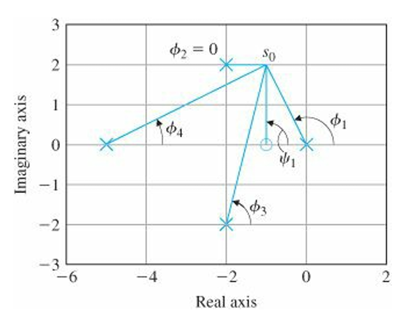
we must have $\angle L(s_0)=180^{\circ}+360^{\circ}(l-1)$ for some integer $l$.
$$\angle(s_0+1)-\angle s_0-\angle(s_0+5)-\angle[(s_0+2)^2+4]=180^{\circ}+360^{\circ}(l-1)$$
$$\angle L=\psi_1-\phi_1-\phi_2-\phi_3-\phi_4=90^{\circ}-116.6^{\circ}-0^{\circ}-76^{\circ}-26.6^{\circ}=-129.2^{\circ}$$
Since the phase of $L(s)$ is not $180 ^{\circ}$, we conclude that $s_0$ is not on the root locus.
Rules for Plotting a Positive($180 ^{\circ} $) Root Locus
Rule 1. The $n$ branches of the locus start at the poles of $L(s)$ and $m$ of these branches end on the zeros of $L(s)$.
Rule 2. The loci are on the real axis to the left of an add number of poles and zeros.
Rule 3. For large $s$ and $K$, $n-m$ of the loci are asymptotic to lines at angles $\phi_l$ radiating out from the point $s=\alpha$ on the real axis where $$\phi_l=\frac{180^{\circ}+360^{\circ}(l-1)}{n-m},\quad l=1,2,...,n-m,\quad\alpha=\frac{\sum p_i-\sum z_i}{n-m}$$
Rule 4. The angle(s) of departure of a branch of the locus from a pole of multiplicity q is given by $$q\phi_{l,dep}=\sum\psi_i-\sum_{i\neq l}^{}\phi_i-180^{\circ}-360^{\circ}(l-1)$$ and the angle(s) of arrival of a branch at a zero of multiplicity q is given by $$q\psi_{l,arr}=\sum\phi_i-\sum_{i\neq l}^{}\psi_i+180^{\circ}+360^{\circ}(l-1)$$
Rule 5. The locus can have multiple roots at points on the locus and the branches will approach a point of q roots at angles separated by $$\frac{180^{\circ}+360^{\circ}(l-1)}{q}$$ and will depart at angles with the same separation.
Selecting the Parameter Value
for $s_0$ on the Root Locus, $$K=-\frac{1}{L(s_0)}=\frac{1}{\left| L(s_0) \right|}$$
e.g.
PD Control with the plant of $$K=\frac{1}{L(s_0)}=\frac{1}{\left| L(s_0) \right|}$$
characteristic eqn: $$1+[k_p+k_Ds]\frac{1}{s^2}=0$$
Let $K=k_D$ and the gain ratio as $\frac{k_p}{k_D}=1$. It results in $$1+K\frac{s+1}{s^2}=0$$
MATLAB code to plot the locus:
numS = [1 1];
denS = [1 0 0];
sysS = tf(numS,denS);
rlocus(sysS)
Effect of a Zero in the LHP
The addition of the zero has pulled the locus into the LHP, a point of general importance in constructing a compensation.
The physical operation of differentiation is not practical. In practice PD control is approximated by $$D(s)=k_p+\frac{k_Ds}{s/p+1}$$
Let $K=k_p+pk_D$, $z=pk_p/K$, then $$D(s)=K\frac{s+z}{s+p}$$
This controller transfer function is called lead compensator
characteristic eqn for the $1/s^2$ plant: $$1+D(s)G(s)=1+KL(s)=1+K\frac{s+z}{s^2(s+p)}=0$$
ex 5.4)
$z=1$, $p=12$
$$1+K\frac{s+1}{s^2(s+12)}=0$$
numL = [1 1];
denL = [1 12 0 0];
sysL = tf(numL,denL);
rlocus(sysL)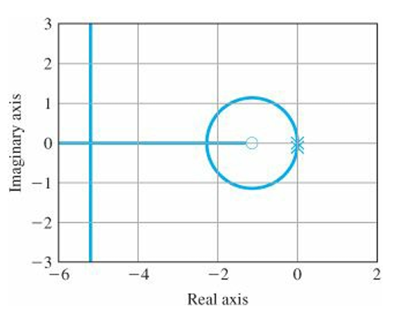
the effect of the added pole has been to distort the simple circle of the PD control
for points near the origin, the locus is quite similar to the earlier case
the situation changes when the pole is brought closer in
ex 5.5)
$z=1$, $p=4$
$$1+K\frac{s+1}{s^2(s+4)}=0$$
numL = [1 1];
denL = [1 4 0 0];
sysL = tf(numL,denL);
rlocus(sysL)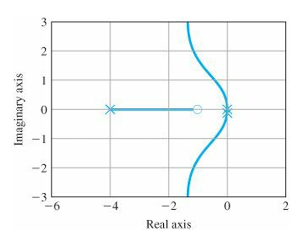
there were both a break-in and a breakaway on the real axis in the case of $p=12$, but these features have disappeared in the case of $p=4$
ex 5.6)
$z=1$, $p=9$
$$1+K\frac{s+1}{s^2(s+9)}=0$$
numL = [1 1];
denL = [1 9 0 0];
sysL = tf(numL,denL);
rlocus(sysL)
When the third pole is near the zero (p near 1), there is only a modest distortion of the locus that would result for $D(s)G(s)\cong K\frac{1}{s^2}$ which consists of two straight-line locus branches departing at $\pm90^\circ$ from the two poles at $s = 0$.
As we increase p, the locus changes until at $p = 9$ the locus breaks in at –3 in a triple multiple root.
As the pole p is moved to the left beyond –9, the locus exhibits distinct break-in and breakaway points, approaching, as p gets very large, the circular locus of one zero and two poles.
When p = 9, is thus a transition locus between the two second-order extremes, which occur at p = 1 (when the zero is canceled) and p → ∞ (where the extra pole has no effect).
Design using Dynamic Compensation
Lead compensation approximates the function of PD control and acts mainly to speed up a response by lowering rise time and decreasing the transient overshoot.
Lag compensation approximates the function of PI control and is usually used to improve the steady-state accuracy of the system.
Notch compensation will be used to achieve stability for systems with lightly damped flexible modes, as we saw with the satellite attitude control having noncollocated actuator and sensor.
Lead and Lag Compensation
$$D(s)=K\frac{s+z}{s+p}$$
Compensation with this transfer function is called Lead Compensation if $z<p$ and Lag Compensation if $z>p$.
Compensation is typically placed in series with the plant in the feed-forward path.
It can also be placed in the feedback path and in that location has the same effect on the overall system poles but results in different transient responses from reference inputs.
characteristic eqn: $$1+D(s)G(s)=1+KL(s)=0$$

Lead Compensation
e.g.
$$G(s)=\frac{1}{s(s+1)}$$
$D(s)=K$(solid) vs. $D(s)=K(s+2)$(dashed)

The effect of the zero is to move the locus to the left, toward the more stable part of the s-plane.
If our speed-of-response specification calls for $\omega_n=2$, then proportional control alone (D = K) can produce only a very low value of damping ratio $\zeta$ when the roots are put at the required value of $\omega_n$.
But, the pure derivative control is not normally practical because of the amplification of sensor noise implied by the differentiation and must be approximated. If the pole of the lead compensation is placed well outside the range of the design $\omega_n$, then we would not expect it to upset the dynamic response of the design in a serious way. $$D(s)=K\frac{s+2}{s+p}$$
Consider $p=10$ and $p=20$.

For small gains, before the real root departing from –p approaches –2, the loci with lead compensation are almost identical to the locus for pure PD. The effect of the pole is to lower the damping, but for the early part of the locus, the effect of the pole is not great if $p > 10$.
In general, the zero is placed in the neighborhood of the closed-loop $\omega_n$, as determined by rise-time or settling-time requirements, and the pole is located at a distance 5 to 20 times the value of the zero location. The choice of the exact pole location is a compromise between the conflicting effects of noise suppression, for which one wants a small value for p, and compensation effectiveness for which one wants a large p. In general, if the pole is too close to the zero, the root locus moves back too far toward its uncompensated shape and the zero is not successful in doing its job. On the other hand, when the pole is too far to the left, the magnification of sensor noise appearing at the output of D(s) is too great and the motor or other actuator of the process can be overheated by noise energy in the control signal, $u(t)$. With a large value of p, the lead compensation approaches pure PD control.
ex 5.11)
Find a compensation for $G(s) = \frac{1}{s(s+1)}$ that will provide overshoot of no more than 20% and rise time of no more than 0.3 sec.
Note that $M_p$(overshoot) is the maximum amount of the overshoot divided by the final value where $M_p=y(t_p)-1=e^{-\sigma\pi/\omega_d}=e^{-\pi\zeta/\sqrt{1-\zeta^2}}$ and $t_r$(rise time) is the time to reach the vicinity of the new set point where $t_r\approx \frac{1.8}{\omega_n}$
So, the requirement is $\zeta\geq 0.5$ and $\omega_n\cong \frac{1.8}{0.3}=6$.
To provide some margin, we'll shoot for $\zeta\geq 0.5$ and $\omega_n\geq 7 rad/sec$.
Let's try with $$D(s)=K\frac{s+2}{s+10}$$
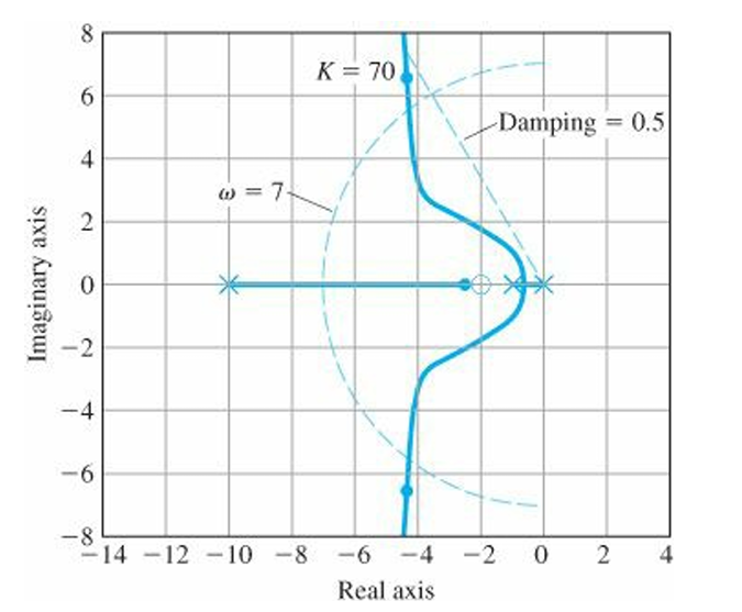
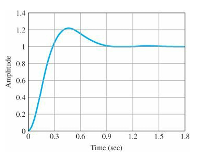
$K = 70$ yields $\zeta = 0.56$ and $\omega_n = 7.7 rad/sec$
But the step response of the system exceeds the overshoot specification a small amount.
Typically, lead compensation in the feed forward path will increase the step-response overshoot because the zero of the compensation has a differentiating effect.
We can tune the compensator to achieve better damping in order to reduce the overshoot in the transient response using RLTOOL.
sysG=tf(1,[1 1 0]);
sysD=tf([1 2],[1 10]);
rltool(sysG,sysD)
By moving the pole of the lead compensator more to the left in order to pull the locus in that direction, and selecting K = 91, we obtain $$D(s)=91\frac{s+2}{s+13}$$


The phase at $s=j\omega$ is given by $$\phi=\tan^{-1}\left ( \frac{\omega}{z} \right )-\tan^{-1}\left ( \frac{\omega}{p} \right )$$
If $z < p$, then $\phi$ is positive, which by definition indicates phase lead.
Lag Compensation
Once satisfactory dynamic response has been obtained, perhaps by using one or more lead compensations, we may discover that the low-frequency gain—the value of the relevant steady-state error constant, such as $K_v$—is still too low.
The system type, which determines the degree of the polynomial the system is capable of following, is determined by the order of the pole of the transfer function $D(s)G(s)$ at $s = 0$. If the system is Type 1, the velocity-error constant, which determines the magnitude of the error to a ramp input, is given by $\displaystyle \lim_{s \to 0}sG(s)D(s)$.
In order to increase this constant, it is necessary to do so in a way that does not upset the already satisfactory dynamic response. Thus, we want an expression for $D(s)$ that will yield a significant gain at s = 0 to raise $K_v$ (or some other steady-state error constant) but is nearly unity (no effect) at the higher frequency $\omega_n$, where dynamic response is determined. The solution is lag compensation. $$D(s)=\frac{s+z}{s+p},\quad z>p$$
The values of z and p are small compared with $\omega_n$, yet $D(0) = \frac{Z}{p} = 3\;to\;10$ (the value depending on the extent to which the steady-state gain requires boosting) Because z > p, the phase $\phi$ is negative, corresponding to phase lag.
e.g.
Consider $$G(s)=\frac{1}{s(s+1)}$$
with lead compensator $$KD_1(s)=K\frac{s+2}{s+13}$$
with the gain of $K=91$ from the previous example, the velocity constant is $$K_v=\displaystyle \lim_{s \to 0}sKD_1G=\displaystyle \lim_{s \to 0}s(91)\frac{s+2}{s+13}\frac{1}{s(s+1)}=\frac{91*2}{13}=14$$
Suppose we require that $K_v = 70$. To obtain this, we require a lag compensation with $Z/p = 5$ in order to increase the velocity constant by a factor of 5. This can be accomplished with a pole at $p= -0.01$ and a zero at $z = -0.05$, which keeps the values of both z and p very small so that $D_2(s)$ would have little effect on the portions of the locus representing the dominant dynamics around $\omega_n=7$. The lag compensation transfer function is $$D_2(s)=\frac{s+0.05}{s+0.01}$$
$$KD(s)=91\frac{s+2}{s+13}\frac{s+0.05}{s+0.01}$$
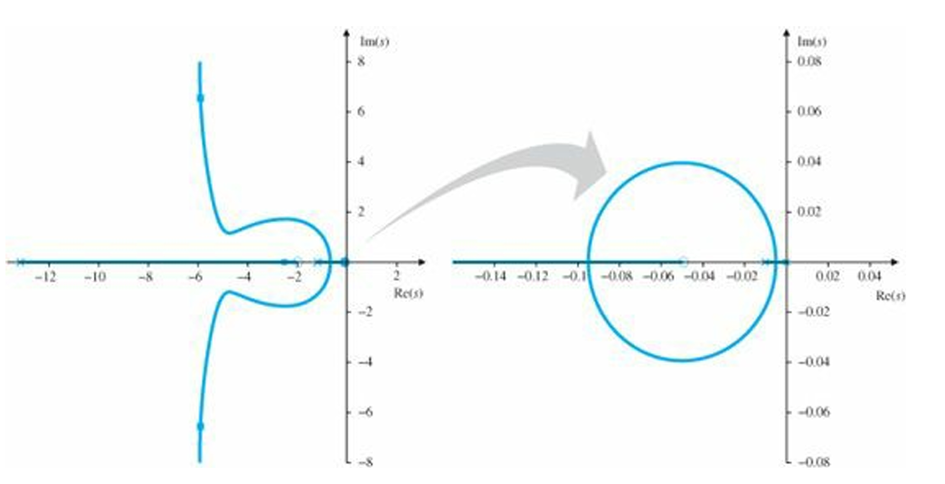
With $K = 91$, the dominant roots are at $-5.8 \pm j6.5$. The effect of the lag compensation can be seen by expanding the region of the locus around the origin(right side of the figure above). The circular locus is a result of the small pole and zero. The transient response corresponding to this root will be a very slowly decaying term, which will have a small magnitude because the zero will almost cancel the pole in the transfer function. The decay is so slow that this term may seriously influence the settling time, and zero will not be present in the step response to a disturbance torque and the slow transient will be much more evident there. That's why it is important to place the lag pole-zero combination at as high a frequency as possible without causing major shifts in the dominant root locations.
Notch Compensation
The lead and lag compensation above is found to have a substantial oscillation at about 50 rad/sec when tested, because there was an unsuspected flexibility of the noncollocated type at a natural frequency of $\omega_n=50$. On reexamination, the plant transfer function, including the effect of the flexibility, is estimated to be $$G(s)=\frac{2500}{s(s+1)(s^2+s+2500)}$$
the very lightly damped roots at 50 rad/sec have been made even less damped or perhaps unstable by the feedback. The best method to fix this situation is to modify the structure so that there is a mechanical increase in damping. Unfortunately, this is often not possible because it is found too late in the design cycle.
How to correct this oscillation?
approach 1) Gain Stabilization: reducing the gain at high frequency
add lag compensation
it might lower the loop gain far enough that there is greatly reduced spillover and the oscillation is eliminated.
approach 2) Phase Stabilization
add a zero near the resonance
this approach can be used if the response time resulting from gain stabilization is too long.
it shifts the departure angles from the resonant poles so as to cause the closed-loop root to move into the LHP, thus causing the associated transient to die out. the result is called a notch compensation which has a transfer function of $$D_{notch}(s)=\frac{s^2+2\zeta\omega_0s+\omega_0^2}{(s+\omega_0)^2}$$
A necessary design decision is whether to place the notch frequency above or below that of the natural resonance of the flexibility in order to get the necessary phase. A check of the angle of departure shows that with the plant compensated and the notch as given, it is necessary to place the frequency of the notch above that of the resonance to get the departure angle to point toward the LHP. Thus the compensation is added with the transfer function $$D_{notch}(s)=\frac{s^2+0.8s+3600}{(s+60)^2}$$
When considering notch or phase stabilization, it is important to understand that its success depends on maintaining the correct phase at the frequencyofthe resonance. If that frequency is subject to significant change, which is common in many cases, then the notch needs to be removed far enough from the nominal frequency in order to work for all cases. The result may be interference of the notch with the rest of the dynamics and poor performance. As a general rule, gain stabilization is substantially more robust to plant changes than is phase stabilization.
'Study > Control' 카테고리의 다른 글
| State-Space Design (0) | 2025.01.30 |
|---|---|
| Frequency-Response Design (0) | 2025.01.15 |
| PID Control (1) | 2025.01.04 |
| Laplace Transform & Transfer Function (0) | 2025.01.04 |
| Introduction: the Fundamentals of Control Theory (0) | 2024.12.28 |