Proportional Control (P)
Feedback control signal is linearly proportional to the system error.
$$\frac{U(s)}{E(s)}=D_{cl}(s)=k_p$$
e.g. second order plant for a motor with nonnegligible inductance
Plant transfer function: $$G(s)=\frac{A}{s^2+a_1s+a_2}$$
Characteristic eqn: $$1+k_pG(s)=0\;\to\; s^2+a_1s+a_2+k_pA=0$$
- it can determine the natural frequency (constant term in eqn)
- it can't determine the damping
- system type 0
- if $k_p$ is made large to get adequately small steady-state error, the damping may be much too low for satisfactory transient response with proportional control alone.
Proportional Plus Integral Control (PI)
Add an integral term to the controller to get the automatic reset effect results in the proportional plus integral control equation in the time domain.
$$u(t)=k_pe+k_I\int_{t_0}^{t}e(\tau)d\tau$$
$$\frac{U(s)}{E(s)}=D_{cl}(s)=k_p+\frac{k_I}{s}$$
- system type 1
- reject completely constant bias disturbances
e.g.
plant: $$Y=\frac{A}{\tau s+1}(U+W)$$
transform eqn for controller: $$U=k_p(R-Y)+k_I\frac{R-Y}{s}$$
$$(\tau s+1)Y=A(k_p+\frac{k_I}{s})(R-Y)+AW\to(\tau s^2+(Ak_p+1)s+Ak_I)Y=A(k_ps+k_I)R+sAW$$
characteristic eqn: $$\tau s^2+(Ak_p+1)s+Ak_I=0$$ two roots may be complex, $\omega_n=\sqrt{\frac{Ak_I}{\tau}},\;\zeta =\frac{Ak_p+1}{2\tau\omega_n} $
e.g.
plant: $$G(s)=\frac{A}{s^2+a_1s+a_2}$$
characteristic eqn: $$1+(k_p+\frac{k_I}{s})G(s)=0\quad\to\quad s^3+\underbrace{\:a_1s^2\:}_{out\:of\:control}+(a_2+Ak_p)s+Ak_I=0$$
PID Control
An important effect of the D term: providing a sharp response to suddenly changing signals


e.g. plant: $$G(s)=\frac{A}{s^2+a_1s+a_2}$$
characteristic eqn: $$1+(k_p+\frac{k_I}{s}+k_Ds)G(s)=0\quad\to\quad s^3+(a_1+Ak_D)s^2+(a_2+Ak_p)s+Ak_I=0$$
$\to$ three parameters can be determined
Ziegler-Nichols Tuning of the PID Controller
Step response of process control system: process reaction curve as below:

$$\frac{Y(s)}{U(s)}=\frac{Ae^{-st_d}}{\tau s+1}$$
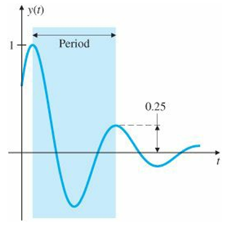
1. Tuning by decay ratio of 0.25
desigining goal: closed-loop step response transient with a decay ratio of approximately 0.25 (corresponding to $\zeta=0.21$)
2. Tuning by evaluation at limit of stability (ultimate sensitivity method)
Criteria for adjusting the parameters are based on evaluating the amplitude and frequency of the oscillations of the system at the limit of stability
The proportional gain is increased until the system becomes marginally stable and continuous oscillations just begin with amplitude limited by the saturation of the actuator. The corresponding gain is defined as $K_u$ (called the ultimate gain) and the period of oscillation is $P_u$ (called the ultimate period).
$P_u$ should be measured when the amplitude of oscillation is as small as possible.
$$D_c(s)=k_p(1+\frac{1}{T_Is}+T_Ds)$$


'Study > Control' 카테고리의 다른 글
| State-Space Design (0) | 2025.01.30 |
|---|---|
| Frequency-Response Design (0) | 2025.01.15 |
| Root Locus, Compensation (0) | 2025.01.13 |
| Laplace Transform & Transfer Function (0) | 2025.01.04 |
| Introduction: the Fundamentals of Control Theory (0) | 2024.12.28 |